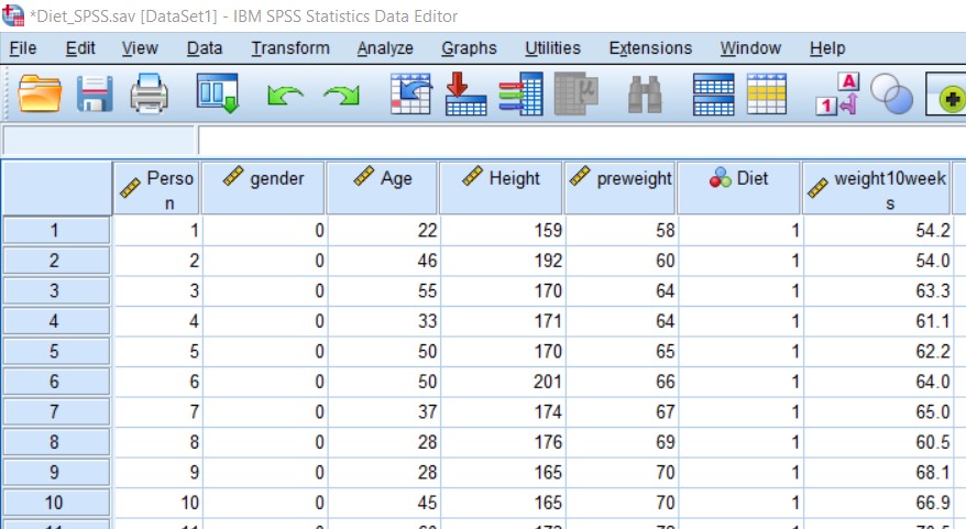
Data manipulation is half of the analysis. Data manipulation means editing the data such as sorting, recoding the existing variables into new, adding labels to the data, inserting the new data, changing a specific value and many others. Some people do the data manipulation in Excel and then reopen it in SPSS for analysis. This is not prohibited however a little bit inefficient. A typical data sheet looks like below:

Sorting the data
Sorting the data means arranging the data in ascending (smallest to largest) or descending (largest to smallest) order. You can sort data by a single or multiple variable. Sorting the data by a specific variable will change all other variables accordingly. This is a very helpful tool for exploring the data. You can sort the data by the variable ‘Person’ in ascending order using following command line.
| Data – Sort cases | Command 3 |
Which will open a new window where you will select the variable by which you would like to sort the data set. Then select the option ascending or descending and click ok button. By sorting you can explore the outliers, missing values, or any unusual values in the data set. Sort person ID, age and gender and see if you find anything.
In the menu Data you can many other options for exploring data such as identifying duplicate observation, identifying missing observations, merging variables and variables etc.
Creating new variable
You will need to create new variable using existing variable frequently. You can simply do that in SPSS.
Let us use the diet data where we have weight in kg of some people before and after 10 weeks of following a specific diet. We want to create a new variable the amount of weight lost after 10 weeks of that specific diet. We can do that using the following command line.
| Transform – Compute variable | Command 4 |
This will open a new dialog box where you will have to do some arithmetic. In the Target Variable box you have to give a name for the new variable, for example ‘wt_loss’, in the Numeric Expression box do the arithmetic using existing variable, for example the ‘preweight’ and ‘weight10weeks’ for the diet data. Once you wrote the numerical expression click the ok button that will generate the desired variable and will be added to the data set.
Exercise 1.1: Calculate the BMI [BMI = weight(kg)/height(m)2] from the diet data.
Another case of generating new variable which is more useful. Let us assume our target was to lose 3 kg of weight in 10 weeks. Now we want to create a binary variable which will have two values 0(weight loss less than 3kg) and 1(weight loss 3kg or more). We can do that using the following command line.
| Transform – Recode into different variables | Command 5 |
There will be a new dialog box open. In the input output variable box, add the variable that you want to recode, in this case it will be ‘wt_loss’. Give a name of the new variable in the output variable box with or without a label, for example ‘wt_loss_bin’. Then click change button. Click old and new values which will open a new window where there will be two box, old value and new value. You can provide a single value or a range of values. In this case, we will provide range lowest through 3 in old value and 0 in new value, a range 3 through highest in new value and 1 in new value. Then press the continue and click ok button. This will generate the new variable and added to the data set. You can change the label of 0 and 1 from the variable view, in column values.


Leave A Comment